Predicting whether a person has a ‘Heart Disease’ or ‘No Heart Disease’. This is an example of Supervised Machine Learning as the output is already known.

It is a Classification Problem. As we have to classify the outcome into 2 classes:

1(ONE) as having Heart Disease and

0(Zero) as not having Heart Disease.

Where to get the Dataset

Heart Disease is a data set available in UCI repository as well as can be downloaded from Kaggle the link is provided below:

https://www.kaggle.com/priyanka841/heart-disease-prediction-uci

DataSet Description

There are 14 features(Columns) including the target. The data set includes features like:

• slope_of_peak_exercise_st_segment (type: int): the slope of the peak exercise ST segment, an electrocardiography read out indicating quality of blood flow to the heart
• thal (type: categorical): results of thallium stress test measuring blood flow to the heart, with possible values normal, fixed_defect, reversible_defect
• resting_blood_pressure (type: int): resting blood pressure
• chest_pain_type (type: int): chest pain type (4 values)
• num_major_vessels (type: int): number of major vessels (0-3) colored by flourosopy
• fasting_blood_sugar_gt_120_mg_per_dl (type: binary): fasting blood sugar > 120 mg/dl
• resting_ekg_results (type: int): resting electrocardiographic results (values 0,1,2)
• serum_cholesterol_mg_per_dl (type: int): serum cholestoral in mg/dl
• oldpeak_eq_st_depression (type: float): oldpeak = ST depression induced by exercise relative to rest, a measure of abnormality in electrocardiograms
• sex (type: binary): 0: female, 1: male
• age (type: int): age in years
• max_heart_rate_achieved (type: int): maximum heart rate achieved (beats per minute)
• exercise_induced_angina (type: binary): exercise-induced chest pain (0: False, 1: True)

Let’s Now Start the Data Loading

Checking the Null Values and we find that we do not have any null values in the dataset.

We find that we do not have null values, and hence it is not required on our part to fill these values. The data type is numeric for all the features, this implies that we do not have to change the data into dummy variables or apply one hot encoding etc. before applying any algorithm.

You can access the Jupyter Notebook here:

file:///C:/Users/HP/Downloads/Heart%20Disease.html

Well , let’s move on further with Data Visualization and Analysis

Box and Whiskers plot are useful to find out outliers in our data. If we have more outliers we will have to remove them or fix them; otherwise they will become as noise for the training data.

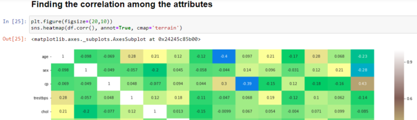
Let’s Visualize the features and their relation with the target( Heart Disease or No Heart Disease)

we do scaling to bring all the values to the same magnitude. Scaling or Standardization is brings the mean to zero and standard deviation to ‘one’. It assumes a Gaussian distribution. We perform Scaling to avoid biased predictions.

Comparison Between Unscaled and Scaled DataFrame

Next let us prepare our data for Training

Applying Logistic Regression Algorithm and finding the accuracy, precision and recall of the model.

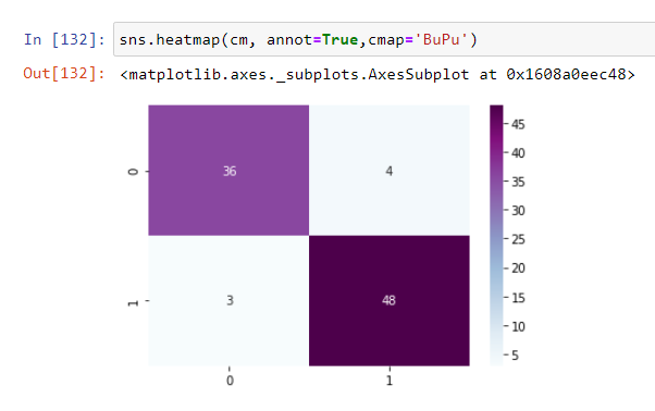
Precision is the fraction of heart diseases that were predicted to be heart diseases and were actually heart diseases.

Whereas, Recall measures the fraction of true cases of Heart Disease that were detected. It also takes into account those values which were incorrectly rejected by the algorithm. We observe that the recall for ‘1’ i.e having heart disease is higher that means that the algorithm is incorrectly rejecting a few cases.

The formula is given by:

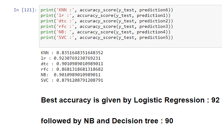
I have performed the similar test on various algorithms and found that Logistic Regression followed by Naive Bayes are giving good accuracy with 92% and 90% respectively.