
This blog will address how to get started with Time Series Analysis in Python. We will work with TCS data se, the file can be downloaded from the link below. There are around 52 files in this zip folder, select TCS.csv file to get started with the analysis.
https://www.kaggle.com/rohanrao/nifty50-stock-market-data
Time Series Analysis
Time series Analysis is a statistical technique that deals with data in series of particular time periods or intervals. Previous values of the series is used to predict the future value. Time Series analysis can be useful to see how a given asset, security or economic variable changes over time. It is also used to examine how the changes associated with the chosen data point compare to shifts in other variables over the same time period. Don’t worry just get a general idea as this will become clear with example.
For example, suppose you wanted to analyze a time series of daily closing stock prices for a given stock over a period of one year. You would obtain a list of all the closing prices for the stock from each day for the past year and list them in chronological order. This would be a one-year daily closing price time series for the stock.
Time Series Forecasting
Time series forecasting uses information regarding historical values and associated patterns to predict future activity. Most often, this relates to trend analysis, cyclical fluctuation analysis, and issues of seasonality.
Examples of Time Series Analysis
- Wind Speed
- Power Prediction
- Stock Market Prediction
- Weather Prediction
Why do we need Time Series Analysis
We notice that everything changes with respect to time. Be it customer preferences, Stock prices, weather conditions, economic factors, global situations, international and national situations like recession, unemployment, volatility, growth and so on. Thus, in such changing and dynamic conditions we need to
- Better understand the changes
- Understand how the changes have impacted the scenario
- Based on the analysis draw insights, improve decisions
Components of Time Series
- Trend Component: This is a variation that moves up or down in a reasonably predictable pattern over a long period.
- Seasonality Component: is the variation that is regular and periodic and repeats itself over a specific period such as a day, week, month, season, etc.,
- Cyclical Component: is the variation that corresponds with business or economic ‘boom-bust’ cycles or follows their own peculiar cycles, and
- Random Component: is the variation that is erratic or residual and does not fall under any of the above three classifications.
To make this concept more clear here is a visual interpretation of the various components of the Time Series. You can view the original diagram with its context, here.

Dataset
In this blog, we will use TCS data set to analyze stock prices and perform some basic time series operations. Tata Consultancy Services Limited (TCS) is an Indian multinational information technology (IT) services and consulting company. It is a subsidiary of the Tata Group and operates in 149 locations across 46 countries. Its market Valuation is of Rs 9 lakh crore (second only after Reliance).

Let us get Started with the Time Series Analysis
We will start with loading basic libraries, data set and will have a look at the dataset. The slideshow will display the code snippets.

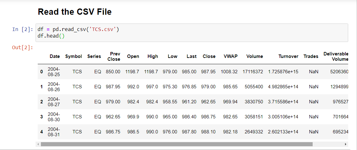


The dataset has over 3900 rows and 15 columns. Date here is recognized as an object data type and not as dates. Thus, we need pandas to_datetime() feature which converts the arguments to dates. Further, for the sake of convenience and analysis, we will use a dataset with few columns (7 columns)


Understanding the Stock Data
Let us understand various columns for further analysis.
- The Open and Close columns indicate the opening and closing price of the stocks on a particular day.
- The High and Low columns provide the highest and the lowest price for the stock on a particular day, respectively.
- The Volume column tells us the total volume of stocks traded on a particular day.
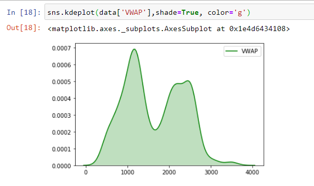
The volume weighted average price (VWAP) is a trading benchmark used by traders that gives the average price a security has traded at throughout the day, based on both volume and price. It is important because it provides traders with insight into both the trend and value of a security.source.
Visualization
We visualize the VWAP of TCS shares and plot VWAP to visualize how the prices and value fluctuate over time.This is a very basic plot, to make it more meaningful let us plot month and year wise trends.

Subsetting Data Using Pandas Dataframes
Instead of working with the entire data, we will work with the volume weighted average price (VWAP), as VWAP is a trading benchmark. It is possible to slice the Time Series data to highlight the portion of the data we are interested in, hence working with a selected column becomes easier. Further, we will plot the month-wise trend of various years and analyse how it impacted the TCS average share prices.


Key Findings
- Month wise trend analysis for the year 2020, we notice that the share prices started to decline in March; that is when the pandemic Corona hit us hard and finally leading to a lockdown.
- The VWAP still was in the range 1600-1800 until May 2020.
- The value of TCS shares picked up after May and is still catching up; seems like we have started to live with Corona and investors sentiments needs to be respected as the share values are rising again.
- Further breaking down the months of march till may we can easily visualize the value and trend of TCS share
Feature Extraction
To understand further let us extract the date and time from Date column. We will extract year, month, day, day of week and Weekday name to be more precise in out analysis. Pandas offer us with this utility to extract all date and time details from the data frame.


Time Resampling
Stock price of a single day is not fit to make any analysis hence we need to aggregate data in some way. Either we aggregate the data based on month,or start of each year, or every quarter. This helps to have an overview of stock prices, trends can be better analysed and decisions can be made.
For this example we will be use resample() function. The pandas library has a resample() function which resamples such time series data. The resample method in pandas is similar to its groupby method as it is essentially grouping according to a certain time span. The resample() function looks like this:


Summary of the above code
data.resample()is used to resample the stock data.- The ‘A’ stands for year-end frequency, and denotes the offset values by which we want to resample the data.
mean()indicates that we want the average stock price during this period.- The ‘M‘ stands for the month end frequency.
Below is a complete list of the offset values. The list can also be found in the pandas documentation.

Time Shifting
Sometimes, we may need to shift or move the data forward or backwards in time. This shifting is done along a time index by the desired number of time-frequency increments.Here is the original dataset before any time shifts.


Key Findings
- Pandas Shift() Function, shifts index by the desired number of periods.This function takes a scalar parameter called a period, which represents the number of shifts for the desired axis.
- This function is beneficial when dealing with time-series data.
- Forward Shift shifts the data forward. We will pass the desired number of periods (or increments) through the shift() function, which needs to be positive value in this case. Let’s move our data forward by one period or index, which means that all values which earlier corresponded to row N will now belong to row N+1.
- Backward Shift shifts our data backwards, the number of periods (or increments) must be negative.
- The opening amount corresponding to 2004-08-25 is now 985.65, whereas originally it was 1008.32
Rolling Window
A rolling mean, or moving average, is a transformation method which helps average out noise from data. It works by simply splitting and aggregating the data into windows according to function, such as mean(), median(), count(), etc. For this example, we’ll use a rolling mean for 7 days.


Key Findings
The first six values have all become blank as there wasn’t enough data to actually fill them when using a window of seven days.
Why use Moving Average or rolling mean ?
It is due to the fact that our data becomes a lot less noisy and more reflective of the trend than the data itself. A moving average is commonly used with time-series data to smooth out short-term fluctuations and highlight longer-term trends or cycles.
In the above plot, we plotted the original data followed by the rolling data for 30 days.
The blue line is the original open price data. The orange line represents the 30-day rolling window and has less noise than the orange line. Something to keep in mind is that once we run this code, the first 29 days aren’t going to have the blue line because there wasn’t enough data to actually calculate that rolling mean
Video explaining Time-Series: https://youtu.be/BJyXe0OYiIg
Sources
These sources were of real help.
https://en.wikipedia.org/wiki/Moving_average
https://www.investopedia.com/terms/t/timeseries.asp
https://www.kaggle.com/parulpandey/getting-started-with-time-series-using-pandas

